Accessible Excel Spreadsheets
Many of the techniques used to create accessible Excel spreadsheets are good formatting practice.
Check your document for accessibility
Note: the example in these steps uses Microsoft Word, but the steps also apply to PowerPoint and Excel. Get more info on Microsoft's accessibility checker.
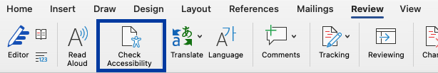
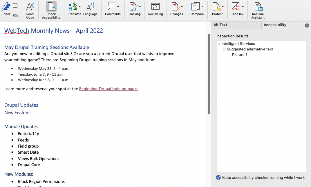
- In the Review tab, choose "Check Accessibility" from the Check Accessibility group.
- An accessibility pane will open, with any errors or warnings to investigate. Use the pane to learn more about an issue and how to fix in the Microsoft product you're using.


Visual Contrast
The easiest way to provide good visual contrast is to leave the entire workbook in black and white.
If color is necessary, you’ll need to test your color contrast ratios. You can download a free Color Contrast Analyzer or access an online Google Chrome: Color Contrast Analyzer plugin.
- Use the foreground eyedropper to select a color in the foreground. Usethe background eyedropper to select a color from the background.
- The analyzer will show the result as “Pass” or “Fail” in the sections labeled (AA) and (AAA).
In order to achieve accessibility compliance our goal is to get a “Pass” in at least the (AA) section.
A “Pass” in the (AAA) section ensures the highest level of compliance.
Worksheet Names and Table Titles
Provide a descriptive name for each worksheet in the workbook. Use a descriptive title for each area of your worksheet that is formatted as a table. Make names and titles descriptive enough that someone, years from now, will understand them.
To center your title above your table:
- Select the cells in the title row corresponding to the width of the table.
- Right click and select the Format Cells option.
- Select the Alignment tab
- Check the Merge Cells box
- In the “Horizontal” alignment drop down, select, Center
- Click Okay
Information in cell A1
- A screen reader starts reading any worksheet from cell A1. If you have a table on the sheet, A1 may simply be the title of the table.
- If the sheet is long or complex, add instructions or an overview of the sheet in cell A1. This will give non-sited users the benefit of knowing what’s being presented and how to use it.
- This instructional text can match the background color. This will hide it from sited users, but allow it to be read by screen readers.
Row and Column Headers
- Each table should have row and column headers that makes sense. Column headers should occupy one row. Don’t leave any headers blank, even if the meaning seems obvious to you.
Avoid Blank Cells
- Cells should never be left blank. If there is no data in a cell, then you should insert a note indicating such, such as, “No data."
- Avoid blank rows and columns.
- If more space is needed for readability, increase the height or width of cells.
- Don’t merge or split cells. The exception to this is for titles above the table.
- If you have two or more tables on a worksheet, you may leave a single blank row between each table.
Hyperlinks
In order for hyperlinks to be accessible we must add a “ScreenTip”. To ensure that your hyperlinks are working properly.
- Right click on the cell containing a URL and choose, Hyperlink or click edit Hyperlink if one is already present.
- Place the full URL in the Address box. Leave the, “Text to Display” box blank, so the URL will display on the spreadsheet.
- Click the ScreenTip button located on the upper right to add a description of what the link leads to.
ScreenTips appear when you mouse over the link, and are readable by screen readers.
Remove Comments
Screen readers are unable to read comments. If the information in comments is important to your audience, place it in a cell.
To remove a comment, Right click on the cell and select “Delete Comment."
Hide Unused Rows and Columns
Screen readers do not read hidden cells. If a cell is hidden from a sited user, it is also hidden from someone using a screen reader.
You can hide rows or columns by right clicking on them and selecting Hide. You can select multiple rows and columns by holding CTRL while clicking. Alternatively, hold Shift+Ctrl and then tap the right arrow key (for columns) or the down arrow key (for rows.)
Images
Ensure that all images have alt text descriptions.
- Right click and choose Size and Properties
- The Format Picture tab will appear. Choose the Alt text tab.
- Type in a brief description with enough detail to explain the picture being displayed.
There is no need to include “image of” or “picture of” in the alt text. The screen reader notifies the user of this information automatically.
Charts
Charts, like images, require alt text. However, unlike images, charts created in Excel don’t have a property for this. To create descriptions for charts:
- Resize/organize the row where you want to insert the chart.
- Insert the chart.
- In the cell(s) where the chart is to be placed, type a description of the chart.
Depending on the complexity of the chart, this description may be lengthy. Provide as much information as needed to sufficiently explain the chart.
- Hide the text of the description by changing its color to match the background. When a screen reader comes across the cell containing the chart, it will read the text description.
Stay in the Grid
Information located in the grid of cells is read in the correct order by screen readers. Information floating on top of the grid, contained in text boxes, charts and images, is read out of place. They are announced as, “Embedded objects," and may lose their context.
If the object has alt text, it will be read by a screen reader. But the screen reader cannot tell where in the grid the object is located or what it may refer to in the grid.
Instead of writing in a text box, put the information in a cell. You will have to design your worksheet so that the text is read in order with respect to the surrounding data.
The alt text of images should explain the relationship of the image to the data presented in the worksheet.
Check Spelling
Perform a spell check on each worksheet. Excel doesn’t put wavy red line under a word it thinks is misspelled. It will only spell check one worksheet at a time.
Under the Review tab in the Proofing group, select Spelling and follow the prompts.
Document Properties
Fill out the document properties following your agency’s standards. This provides background information on the workbook for those reviewing it later. It also assists web searches in locating the document.
- Click the File tab, and choose the Info tab on the left
- On the right there should be a frame listing the properties
- Select Advanced Properties
- Select the Summary tab and enter the information in the form provided
End of Worksheet
Add the text “End of Worksheet” in column A after the last row of data on each worksheet. This lets screen reader users know that there is nothing further to review on the current worksheet.
Set Print Area
- Highlight all information contained within the worksheet
- At the top of your screen select the Page Layout tab
- In the Page Setup group, under Print Area, select Set Print Area
Define the Title Region
This is an important step. Save this step for when you are ready to publish.
The “Title Region” is a little bit of code that lets the screen reader know how to repeat the row and column titles when reading the data. This makes the table easier for users to understand.
- Select the top left cell in your table (excluding the table Title).
- Go to the Formulas tab at the top of your screen and choose Name Manager from the Defined Names group.
- Choose New
- In the “Name” box type:
TitleRegion then put a 1 if this is the first table on your worksheet then a period, then the range of cells in your table from top left to bottom right with a period in between, then another period, followed by the worksheet number.
Example: TitleRegion1.A1-G32.1
- If your table only has one column header, define a ColumnTitleRegion instead of a TitleRegion. The coding procedure is the same as the TitleRegion.
- If your table only has one row header, define a RowTitleRegion. The coding procedure is the same as the TitleRegion.
- Click Okay and Close
Save the File
When you save a file, Excel remembers the last sheet you were working on and the last cell selected on each sheet.
To ensure that screen readers will begin in the A1 cell on each sheet, select that cell in each sheet before you save the file.
Similarly, if you want users to begin at the A1 cell on the first sheet, save the file with that sheet and cell selected.